Introduction

A branch of machine learning models that are built using principles of neuronal organization discovered by connectionism in the biological neural networks constituting animal brains.

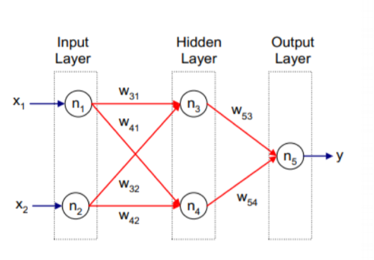
An Artificial Neural Network (ANN) teaches computers to process data inspired by the human brain. It is a type of deep learning that uses nodes or neurons interconnected in a hierarchical structure similar to the human brain. Hidden layers are needed if the data must be separated using a non-linear boundary. Generalize the single neuron perceptron to a more complex architecture of nodes capable of learning nonlinear decision boundaries.

What is the difference between ANN and Perceptron

The major difference is the inclusion of hidden layers. Perceptron can create only one hyperplane.

Structure of ANN

Three kinds of neural networks

1. Feed Forward Neural Networks (FFNN)

General neural networks for classification, regression, etc.

2. Convolutional neural networks

Excel at image recognition.

3. Recurrent neural networks

Excel at language tasks.

Hidden Layer

It can be viewed as learning potential representations or features that are useful to differentiate classes. Also, it dramatically improves their ability to represent arbitrarily complex decision boundaries. Hidden nodes learn potential representation features useful for class boundaries. The first hidden layer captures simpler features since it receives the predictors as input. Subsequent hidden layers hone specific patterns of the data to extract features.

Activation Function

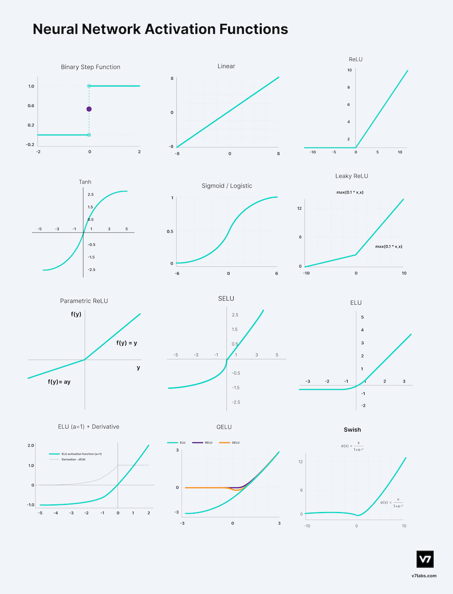
It provides non-linearity to an ANN and allows it to create non-linear class boundaries.

V7 labs

How to choose?

Match the activation function at the output layer based on the type of prediction problem.

- Regression : Linear activation function.

	$$\sigma(z) = z$$

- Binary classification : Sigmoid / Logistic activation function.
	$$\begin{align} \sigma(z) &= \frac{1}{1 + e^{-x}} \\ \sigma^{'}(z) &= \sigma(z) \cdot (1 - \sigma(z)) \end{align}$$

- Multiclass classification : Softmax activation function.

	$$\sigma(z_i) = \frac{e^{z_i}}{\sum_{j = 1}^{k}{e^{z_j}}}, \;\; for \;\; i = 1, \cdots, k \;\; and \;\; z = (z_1, \cdots, z_k) \in R$$

- Multilabel classification : sigmoid activation function.

	$$\begin{align} \sigma(z) &= \frac{1}{1 + e^{-z}} \\ \sigma^{'} &= \sigma(z) \cdot (1 - \sigma(z)) \end{align}$$

- Convolutional Neural Network (CNN) : ReLU activation function.

	$$\begin{align} \sigma(z) &= max(0, z) \\
	\sigma^{'}(z) &= \begin{cases} 1, \;\; if \;\; z > 0 \\ 0, \;\; if \;\; z ≤ 0 \end{cases} \end{align}$$

- Recurrent Neural Network : Tanh and/or Sigmoid activation function.

	$$\begin{align} \sigma(z) &= \frac{e^{z} - e^{-z}}{e^{z} + e^{-z}} \\
	\sigma^{'}(z) &= 1 - tanh^{2}(z) \end{align}$$

For the hidden layers, start with ReLU activation function and move to others if results are sub-optimal.

Example

Use the sigmoid at the hidden layers and the output layer. $\sigma(z) = \frac{1}{1 + e^{-z}}$

Loss : $\frac{1}{2}\sum_{i = 1}^{n}{(\hat{y_i} - y_i)^2}$

Initialize $\vec{w}$
- \[\vec{w} = N(0, \sigma^2)\]
  - if $\sigma^2$ too small : the output will converge to 0
  - if $\sigma^2$ too large : the output will diverge
  - Xavier initialization : $\sigma^2 = \frac{2}{n_in + n_out}$
  - He initialization : $\sigma^2 = \frac{2}{n_in}$

The network input to the neuron : $z = w^Tx = \sum\_{i = 1}^{n}{w_i x_i} = w_1x_1 + \cdots + w_nx_n$

The output from the neuron : $\sigma(w^Tx) = \sigma(z)$

Feed-Forward Neural Network

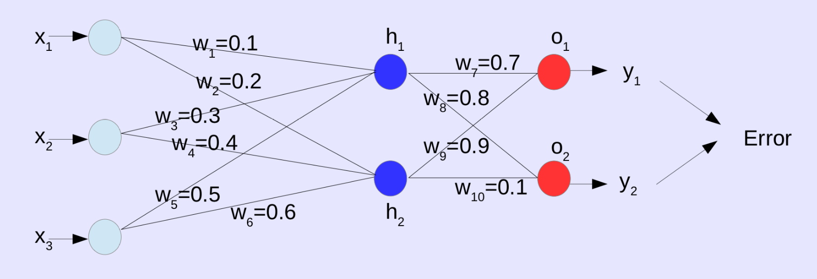
X = [1, 4, 5], y = [0.1, 0.05]

Input for $h_1$ : $z_{h1} = (x_1w_1 + x_2w_3 + x_3w_5) = (1\times0.1) + (4\times0.3) + (5\times0.5) = 3.8$

Output for $h_1$ : $\sigma(z_{h1}) = \sigma(3.8) = \frac{1}{1 + e^{-3.8}} = 0.98$

Input for $h_2$ : $z_{h2} = (x_1w_2 + x_2w_4 + x_3w_6) = (1\times0.2) + (4\times0.4) + (5\times0.6) = 4.8$

Output for $h_2$ : $\sigma(z_{h2}) = \sigma(4.8) = \frac{1}{1 + e^{-4.8}} = 0.99$

Input for $o_1$ : $z_{o1} = (\sigma(z_{h1})\times w_7 + \sigma(z_{h2})\times w_9) = (0.98\times0.7) + (0.99\times0.9) = 1.58$

Output for $o_1$ : $\sigma(z_{o1}) = \sigma(1.58) = \frac{1}{1 + e^{-1.58}} = 0.83$

Input for $o_2$ : $z_{o2} = (\sigma(z_{h1})\times w_8 + \sigma(z_{h2})\times w_{10}) = (0.98\times0.8) + (0.99\times0.1) = 0.88$

Output for $o_2$ : $\sigma(z_{o2}) = \sigma(0.88) = \frac{1}{1 + e^{-0.88}} = 0.71$

Loss: $\frac{1}{2}[(\sigma(z_{o1}) - y_1)^2 + (\sigma(z_{o2}) - y_2)^2] = \frac{1}{2}[(0.83 - 0.1)^2 + (0.71 - 0.05)^2] = 0.48$

Backpropagation

To reduce the loss / error use the Backpropagation method. The chain rule is used for the backpropagation. $\begin{align} \frac{\partial E}{\partial w*7} &= \frac{\partial E}{\partial \sigma(z*{o1})} \cdot \frac{\partial \sigma(z*{o1})}{\partial z*{o1}} \cdot \frac{\partial z*{o1}}{\partial w_7} \\ &= [(\sigma(z*{o1}) - y*1)]\cdot [\sigma(z*{o1})(1 - \sigma(z*{o1}))]\cdot [\sigma(z*{h1})] \\ &= [(0.83 - 0.1)]\cdot [(0.83 - (1 - 0.83)]\cdot [0.98] \\ &= 0.10 \end{align}$ $\frac{\partial E}{\partial w*1} = \frac{\partial E}{\partial \sigma(z*{h1})} \cdot \frac{\partial \sigma(z*{h1})}{\partial z*{h1}} \cdot \frac{\partial z\_{h1}}{\partial w_1}$

Result A gradient vector of weights is used for updating the weights to get to the minimum gradient (Jacobian matrix). $\nabla E = [\frac{\partial E}{\partial w_1}, \frac{\partial E}{\partial w_2}, \frac{\partial E}{\partial w_3}, \frac{\partial E}{\partial w_4}, \cdots, \frac{\partial E}{\partial w_n}]^T = [0.61, 0.87, 0.21, \cdots, 0.99]^T$ Update the weight with this gradient vector: $w_{new} = w_{old} - \eta \nabla E$

Gradient descent

Use gradient descent algorithm for error (or cost) function minimization and to minimize the error function with respect to the weights. This algorithm is used in the training dataset to modify weights during each epoch to minimize the cost or error.

Types

Batch gradient descent : Calculate the error for each observation and perform the update $w$ by calculating the mean error at the end of the training data.
Stochastic gradient descent : Calculate the error for each observation and update $w$.
Mini-batch gradient descent - Preferred method
- Divide the data into small batches, calculate the error for each placed observation, and perform the update $w$ by calculating the mean error at the end of the batch.

Reference

CS 422, Data Mining, prof. Vijay K. Gurbani, Fall 2023, Illinois Institute of Technology